Neural Networks using Keras on Rescale
Rescale now supports running a number of neural network software packages including the Theano-based Keras. Keras is a Python package that enables a user to define a neural network layer-by-layer, train, validate, and then use it to label new images. In this post, we will train a convolutional neural network (CNN) to classify images based on the CIFAR10 dataset. We will then use this trained model to classify new images.
We will be using a modified version of the Keras CIFAR10 CNN training example and will start by going step-by-step through our modified version of the training script.
CIFAR10 Dataset
The CIFAR10 image classification dataset can be downloaded here. It consists of approximately 60000 32×32 pixel images, each given one of 10 categories. You can either download the python version of the dataset directly or use Keras’ built-in dataset downloader (more on this later).
We will load this dataset with the following code:
from keras.datasets import cifar10
from keras.utils import np_utils
nb_classes = 10
def load_dataset():
   # the data, shuffled and split between train and test sets
   (X_train, y_train), (X_test, y_test) = cifar10.load_data()
   print('X_train shape:', X_train.shape)
   print(X_train.shape[0], 'train samples')
   print(X_test.shape[0], 'test samples')
   # convert class vectors to binary class matrices
   Y_train = np_utils.to_categorical(y_train, nb_classes)
   Y_test = np_utils.to_categorical(y_test, nb_classes)
   X_train = X_train.astype('float32')
   X_test = X_test.astype('float32')
   X_train /= 255
   X_test /= 255
   return X_train, Y_train, X_test, Y_test
We are using the cifar10 data loader here, converting the category labels to a one-hot encoding, then scaling the 8-bit RGB values to a 0-1.0 range.
The X_train and X_test outputs are numpy matrices of RGB pixel values for every image in the training and test set. Since there are 50000 training images and 10000 test images and each image is 32×32 pixels with 3 color channels, the shape of each matrix is as follows:
| X_train | (50000, 3, 32, 32) |
| Y_train | (50000) |
| X_test | (10000, 3, 32, 32) |
| Y_test | (10000) |
The Y matrices correspond to an ordinal value representing one of the 10 image classes for the 50000 and 10000 image groups:
| airplane | 0 |
| automobile | 1 |
| bird | 2 |
| cat | 3 |
| deer | 4 |
| dog | 5 |
| frog | 6 |
| horse | 7 |
| ship | 8 |
| truck | 9 |
For the sake of simplicity, we do no further pre-processing on the correctly sized images in this example. In a real image recognition problem, we would do some sort of normalization, ZCA whitening, and/or jittering. Keras integrates some of this pre-processing with the ImageDataGenerator class.
Defining the Network
The next step is to define the neural network architecture we wish to train:
from keras.models import Sequential
from keras.layers.core import Dense, Dropout, Activation, Flatten
from keras.layers.convolutional import Convolution2D, MaxPooling2D
def make_network():
   model = Sequential()
   model.add(Convolution2D(32, 3, 3, border_mode='same',
                           input_shape=(img_channels, img_rows, img_cols)))
   model.add(Activation('relu'))
   model.add(Convolution2D(32, 3, 3))
   model.add(Activation('relu'))
   model.add(MaxPooling2D(pool_size=(2, 2)))
   model.add(Dropout(0.25))
   model.add(Convolution2D(64, 3, 3, border_mode='same'))
   model.add(Activation('relu'))
   model.add(Convolution2D(64, 3, 3))
   model.add(Activation('relu'))
   model.add(MaxPooling2D(pool_size=(2, 2)))
   model.add(Dropout(0.25))
   model.add(Flatten())
   model.add(Dense(512))
   model.add(Activation('relu'))
   model.add(Dropout(0.5))
   model.add(Dense(nb_classes))
   model.add(Activation('softmax'))
   return model
This network has 4 convolutional layers followed by 2 dense layers. Additional layers can be added and layers can be removed or changed, but the first layer must have the same size as an input image (3, 32, 32) and the last dense layer must have the same number of outputs as the number of classes we are using as labels (10). After the final dense layer is a softmax layer that squashes the output to a (0, 1) range that sums to 1.
Training and Testing
Next, we train and test the network:
def train_model(model, X_train, Y_train, X_test, Y_test):
   sgd = SGD(lr=0.01, decay=1e-6, momentum=0.9, nesterov=True)
   model.compile(loss='categorical_crossentropy', optimizer=sgd)
   model.fit(X_train, Y_train, nb_epoch=nb_epoch, batch_size=batch_size,
             validation_split=0.1, show_accuracy=True, verbose=1)
   print('Testing...')
   res = model.evaluate(X_test, Y_test,
                        batch_size=batch_size, verbose=1, show_accuracy=True)
   print('Test accuracy: {0}'.format(res[1]))
Here we have chosen stochastic gradient descent as our optimization method with a cross entropy loss. Then we train the model using the fit() method. We specify the number of training epochs (times we iterate through the data) and the size of our batches (the number of inputs to evaluate on the network at once). Larger batch sizes correspond to more memory usage while training. After our network is trained, we evaluate the model against the test data set and print the accuracy.
Saving the Model
Finally, we save our trained model to files so that we can later re-use it:
def save_model(model):
   model_json = model.to_json()
   open('cifar10_architecture.json', 'w').write(model_json)
   model.save_weights('cifar10_weights.h5', overwrite=True)
Keras distinguishes between saving the model architecture (in our case, what is output from make_network()) and the trained weights. The weights are saved in HDF5 format.
Note that Keras does not guarantee that the saved model is compatible across different versions of Keras and Theano. We recommend you try to load saved models with the same version of Keras and Theano if possible.
Rescale Training Job
Now that we have explained the contents of the cifar10_cnn.py training script we will be running, we will create a Rescale job to train on a GPU node which is already optimized to run on NVIDIA GPUs. This job is publicly available on Rescale. First, we upload the training script and CIFAR10 dataset: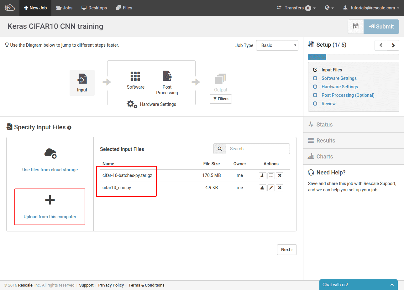
Here we are uploading the pre-processed version of the CIFAR10 images as downloaded by Keras to avoid re-downloading the dataset from the CIFAR site every time the job is run. This step is optional and we could instead just upload the cifar10_cnn.py script.
Next, we select Keras and specify the command line: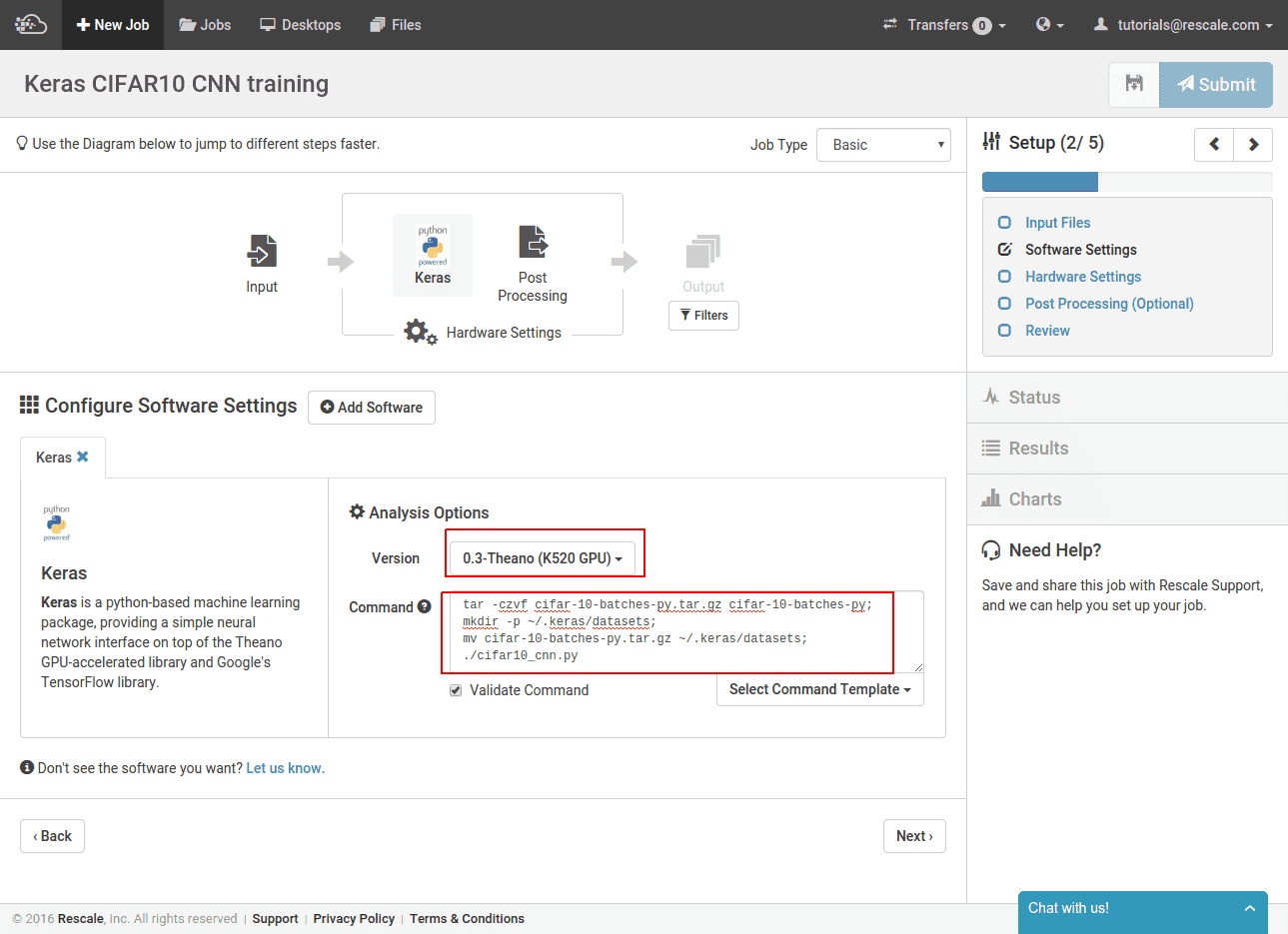
We select Keras from the software picker and then the Theano-backed K520 GPU version of Keras. The command line re-packs the dataset we uploaded and then moves the archive into the default Keras dataset location at ~/.keras/datasets. Then it calls the training script. If we opted to not upload the CIFAR10 set ourselves, we could omit all the archive manipulation commands and just run the training script. The dataset would then be automatically downloaded to the job cluster.
In the last step, we select the GPU hardware we want to run on: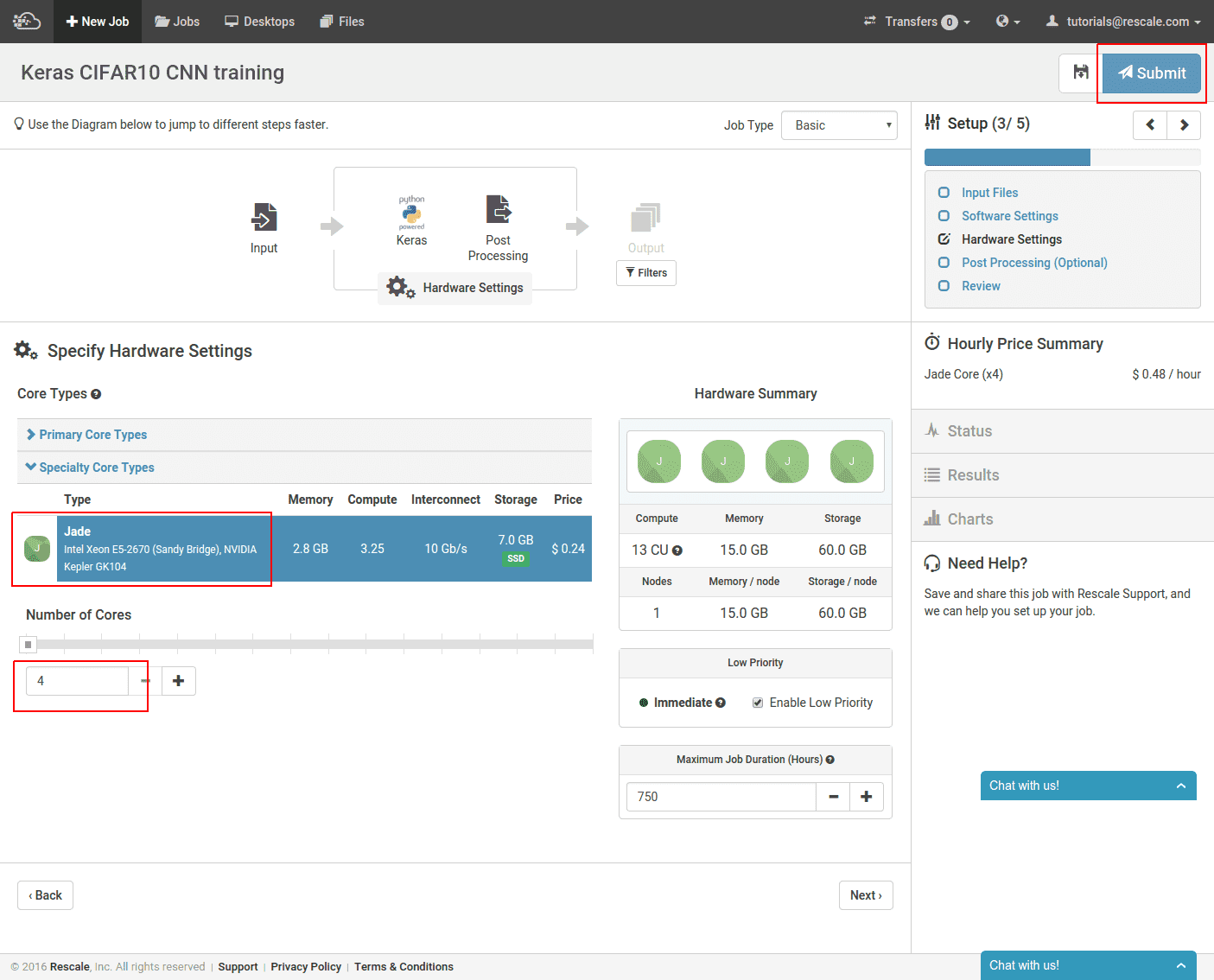
Here we have selected the Jade core type and the minimum 4 cores for this type. Finally, submit the job.
It will take about 15 minutes to provision the cluster and compile the network before training begins. Once it starts, you can view the progress by selecting process_output.log.
Once the job completes, you can use your trained model files. You can either download them from the job results page or use them in a new job, as we will show now.
Classifying New Images
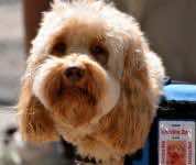
We used a pre-processed numpy-formatted dataset for our training job, so what do we do if we want to take some real images off the internet and classify those? Since dog and cat are 2 of the 10 classes of images represented in CIFAR10, we pick a dog and cat image off the internet and try to classify them: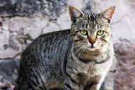
We start by loading and scaling down the images:
import numpy as np
import scipy.misc
def load_and_scale_imgs():
   img_names = ['standing-cat.jpg', 'dog-face.jpg']
   imgs = [np.transpose(scipy.misc.imresize(scipy.misc.imread(img_name), (32, 32)),
                        (2, 0, 1)).astype('float32')
           for img_name in img_names]
   return np.array(imgs) / 255
We use scipy’s imread to load the JPGs and then resize the images to 32×32 pixels. The resulting image tensor has dimensions of (32, 32, 3) and we want the color dimension to be first instead of last, so we take the transpose. Finally, combine the list of image tensors into a single tensor and normalize the levels to be between 0-1.0 as we did before. After processing, the images are smaller:![]()
![]()
Note that we performed the simplest resizing here which does not even preserve the aspect ratio of the original image. If we had done any normalization on the training images, we would also want to apply these transformations to these images as well.
Loading the Model and Labeling
Assembling the saved model is a 2 step process shown here:
from keras.models import model_from_json
def load_model(model_def_fname, model_weight_fname):
   model = model_from_json(open(model_def_fname).read())
   model.load_weights(model_weight_fname)
   return model
Putting it together, we take the model we loaded and call predict_classes to get the class ordinal values for our 2 images.
if __name__ == '__main__':
   imgs = load_and_scale_imgs()
   model = load_model('cifar10_architecture.json', 'cifar10_weights.h5')
   predictions = model.predict_classes(imgs)
   print(predictions)
Rescale Labeling Job
Now to put our labeling script in a job and label our example images. This job is publicly available on Rescale. We start selecting the trained models we created. “Use files from cloud storage” and then select the JSON and HDF5 model files created by the training job: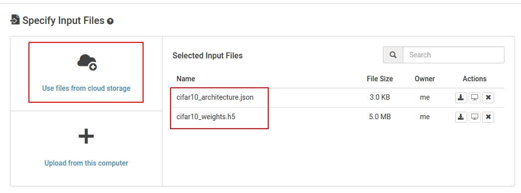
Then upload our new labeling script dog_cat.py and dog and cat images.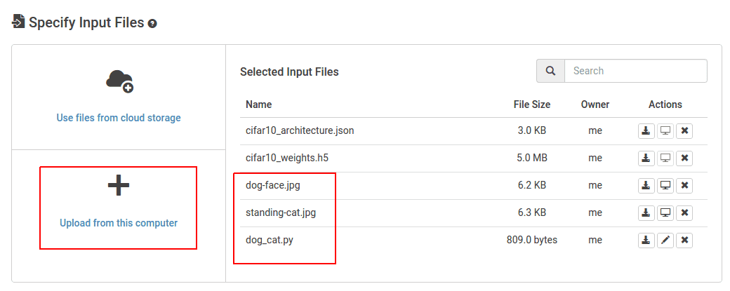
Select the Keras GPU software and run the labeling script. In this case, the dog and cat images are loaded from the current directory where the job is run from, so no files need to be moved around.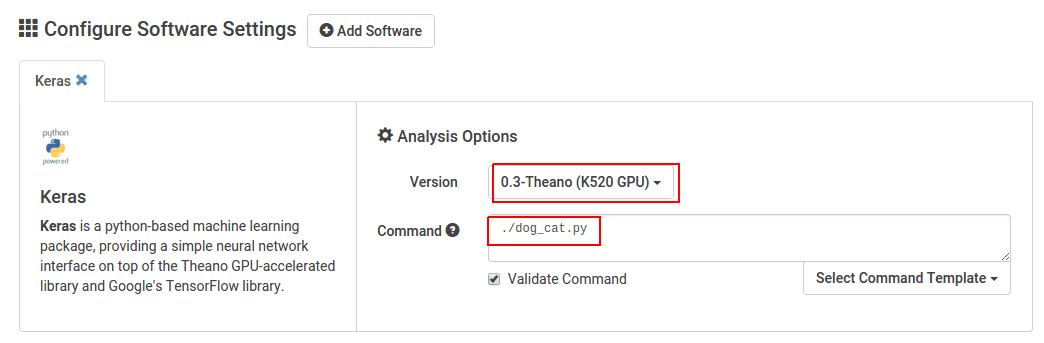
The labels will then be shown in process_output.log when the job completes.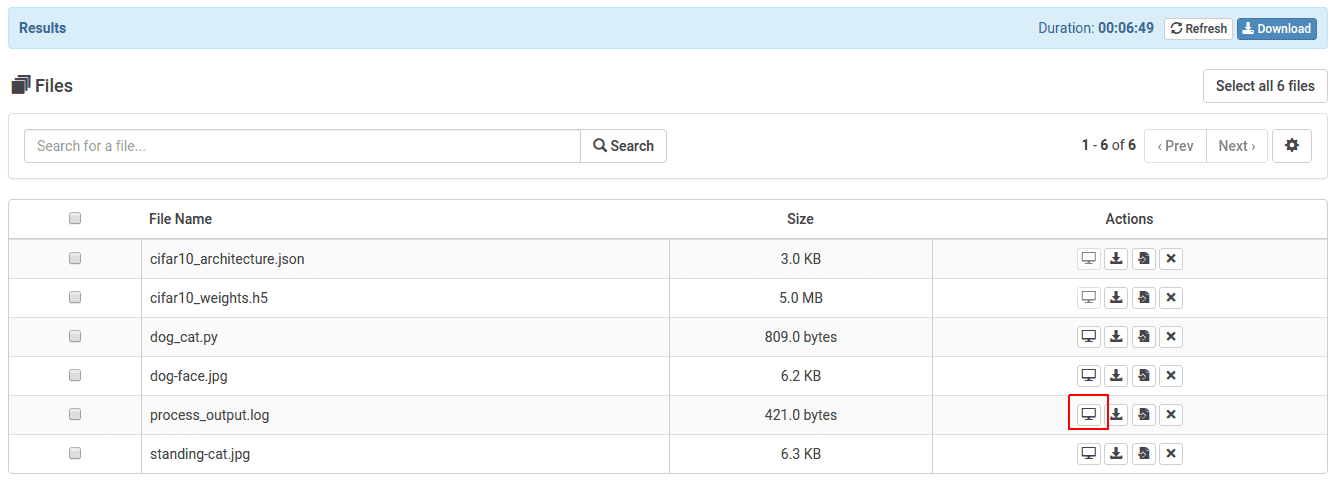
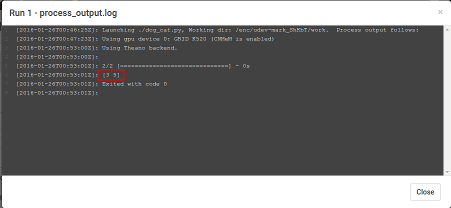
The output is [3, 5] which corresponds to cat and dog from our image class table above.
That wraps up this tutorial. We successfully trained an image recognition convolutional neural network on Rescale and then used that network to label additional images. Coming soon in another post, we will talk about using more complex Rescale workflows to optimize network training.